Supervised Machine Learning Model Evaluation and Selection for Credit Card Fraud Detection
An Overview and purpose:
To evaluate a variety of machine learning algorithms and their ability to correctly identify fraudulent transactions within a population of transactions. The binary classification machine learning models will be evaluated using a labeled dataset consisting of 22 features.
- Trans_date_trans_time: Timestamp of the transaction (date and time).
- Cc_num: Unique customer identification number.
- MerchantThe merchant involved in the transaction.
- Category Transaction type (e.g., personal, childcare).
- Amt: Transaction amount.
- First: Cardholder's first name.
- Last Cardholder's last name.
- Gender: Cardholder's gender.
- Street: Cardholder's street address.
- City: Cardholder's city of residence.
- State: Cardholder's state of residence.
- Zip: Cardholder's zip code.
- Lat: Latitude of cardholder's location.
- Long: Longitude of cardholder's location.
- City_pop: Population of the cardholder's city.
- Job: Cardholder's job title.
- Dob: Cardholder's date of birth.
- Trans_num: Unique transaction identifier.
- Unix_time: Transaction timestamp (Unix format).
- Merch_lat: Merchant's location (latitude).
- Merch_long: Merchant's location (longitude).
- Is_fraud:Fraudulent transaction indicator (1 = fraud, 0 = legitimate). This is the target variable for classification purposes.
The analysis is divided into the following six parts:
- Target variable review.
- Selection of the objective metric(s) for model assessment.
- Feature Engineering and Data Preprocessing.
- Evaluation of various types of machine learning algorithms with minimal tuning.
- Selection of the "best" algorithm from the assessed set of algorithms for hyperparameter tuning.
- Tuning the chosen model for optimal performance.
Part 1 Target Variable Review
The dataset consisted of 555718 transaction records of which 2145 were fraudulent (0.3860%). The labels therefore are highly imbalanced and steps were taken to address the impact of this imbalance on the models.

Part 2 Selection of the objective metric for model assessment
A common metric for machine learning model assessment is accuracy. However, when dealing with a dataset with a highly imbalanced target variable, relying on accuracy for model assessment can cause issues.
Accuracy, as a metric, represents the proportion of correct predictions out of all predictions made. However, when assessing a model’s ability to predict rare positive labels (such as fraudulent transactions), accuracy can be misleading. Why? Because it gives equal weight to both positive (fraudulent) and negative (non-fraudulent) predictions. Let’s illustrate this with an example:
Suppose we have a dataset of 100 transactions, with 50 being fraudulent and 50 non-fraudulent. If a model correctly identifies just 90% of the fraudulent transactions (45 out of 50), it achieves an accuracy score of 95%. However, consider a different scenario: a dataset with only 10 fraudulent records and 90 non-fraudulent records. In this case, the model can achieve the same 90% accuracy by correctly identifying all non-fraudulent transactions but completely missing the fraudulent ones.
Given that our dataset has, on average, only 1 fraudulent transaction for every 259 transactions observed, using accuracy alone as the performance measure is inadequate. To address this, we turn to balanced accuracy.
Balanced accuracy accounts for the class imbalance by considering both positive and negative predictions. It is calculated as the average of two ratios:
The correctly predicted fraudulent transactions are divided by all fraudulent transactions (cpf/af).
The correctly predicted non-fraudulent transactions are divided by all non-fraudulent transactions (cpnf/anf).
Mathematically:
Balanced Accuracy = (cpf/af + cpnf/anf) / 2
Where:
cpf = correctly predicted fraudulent transactions
af = all fraudulent transactions
cpnf = correctly predicted non-fraudulent transactions
anf = all non-fraudulent transactions"
Balanced Accuracy is a more appropriate objective metric over accuracy when working with imbalanced classes in the target, as it weighs each sample according to the inverse prevalence of its true class. It is this metric that is used to assess each model's performance.
Part 3 Feature Engineering and Data Preprocessing
After performing a descriptive analysis of the data some features were dropped or created then encoded/transformed and scaled:
- Dropped Features: 'First' Name, 'Last' Name, 'cc_num', 'street', 'city', 'state', 'dob', 'Trans_num', 'Unix_time', 'Lat', 'Long', 'Merch_lat', 'Merch_long'. The personal identification data was dropped as we didn't want it to influence the analysis, we tried to find the fraudulent customer without knowing their exact ID. Transaction features like Trans_num, and Unix_Time were also dropped as they do not correlate to the inci2ence of fraud.
- Created Features:
- 'Region', an amalgamation of U.S. States according to the U.S. Bureau of Economic Analysis.
- 'Age_years', the age of the cardholder based on the difference between today's date and the cardholder's DOB.
- 'Distance_km', the distance between the cardholder's latitude and longitude and the merchant's latitude and longitude.
Encoding Features with few categories: binary or get_dummies encoding was used to encode categories: 'gender' and 'region'; features with fewer than 20 members.
Transformed Features: 'amt' (Transaction Amount), due to the very high dispersion in this feature it was transformed by the natural log.


Spliting into Training and Testing Sets: The resulting data set was split into training and testing sets with 75% of the data used for training and 25% was used for testing. Due to the very high imbalance in target labels (classes), the training and test splits were reviewed to ensure an adequate number of labels were assigned to each set.
Average class probability in the data set: 0.003860
Average class probability in the training set: 0.003839
Average class probability in the test set: 0.003923The distribution of the y_postive and y_negative labels were reviewed.
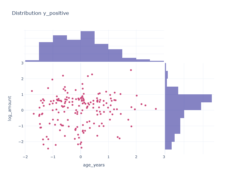
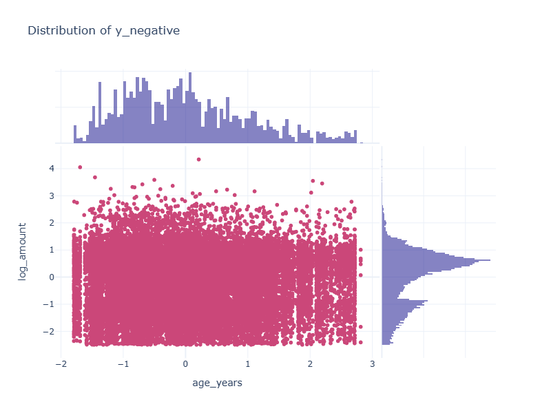
Encoding Features with Extensive Categories: Target encoding was used to encode the 'merchants', and 'jobs' features. It was applied after splitting the data into train and test sets. The target encoder was fit to the training data, the resulting encoder was used to transform both the training and testing sets.
Scaling: Sci-kit Learns standard scaler was fit to the training features, and the training and testing features were transformed with the resulting scaler.
Part 4 Assessing various machine learning algorithms.
The following models were reviewed for their ability to achieve a balanced accuracy score while maximizing the recall of the model.
1. Logistic Regression
| Confusion Matrix | Predicted Legitimate 0 | Predicted Fraudulent 1 | |
|---|---|---|---|
| Legitimate 0 | 138366 | 19 | |
| Fraudulent 1 | 520 | 25 | |
| Accuracy Score: 0.9961 | |||
| Balanced Accuracy Score: 0.5229 | |||
| Classification Report | |||
| Class | Precision | Recall | F1-score |
| 0 | 1.00 | 1.00 | 1.00 |
| 1 | 0.57 | 0.05 | 0.08 |
| Accuracy | 1.00 | ||
| Macro avg | 0.78 | 0.52 | 0.54 |
| Weighted avg | 0.99 | 1.00 | 0.99 |
The logistic regression model as illustrated above has a mediocre performance when attempting to predict the fraudulent records in the test set as evidenced by the recall of 0.05 where approximately 1 in every 20 fraudulent transactions were detected. This low performance is further illustrated by the 0.52 balanced accuracy score achieved. Based on this result we moved on to a non-linear model.
2. Support Vector Machine (Kernel RBF)
| Confusion Matrix | Predicted Legitimate 0 | Predicted Fraudulent 1 | |
|---|---|---|---|
| Legitimate 0 | 138364 | 21 | |
| Fraudulent 1 | 410 | 135 | |
| Accuracy Score: 0.9969 | |||
| Balanced Accuracy Score: 0.6238 | |||
| Classification Report | |||
| Class | Precision | Recall | F1-score |
| 0 | 1.00 | 1.00 | 1.00 |
| 1 | 0.87 | 0.25 | 0.39 |
| Accuracy | 1.00 | ||
| Macro avg | 0.93 | 0.62 | 0.69 |
| Weighted avg | 1.00 | 1.00 | 1.00 |
The non-linear Support Vector Machine model with the non-linear radial bias activation function performs marginally better than the logistic regression function. It yields a 0.10 improvement in the balanced accuracy score and a 5-fold improvement in model recall. However the model is only able to detect 25% of the fraudulent transactions.
3. Random Forest Classifier
| Confusion Matrix | Predicted Legitimate 0 | Predicted Fraudulent 1 | |
|---|---|---|---|
| Legitimate 0 | 138352 | 33 | |
| Fraudulent 1 | 208 | 337 | |
| Accuracy Score: 0.9983 | |||
| Balanced Accuracy Score: 0.8091 | |||
| Classification Report | |||
| Class | Precision | Recall | F1-score |
| 0 | 1.00 | 1.00 | 1.00 |
| 1 | 0.91 | 0.62 | 0.74 |
| Accuracy | 1.00 | ||
| Macro avg | 0.95 | 0.81 | 0.87 |
| Weighted avg | 1.00 | 1.00 | 1.00 |
Next, we reviewed an ensemble random forest model which was much more performant than the previous two models. With this model, we started to see a more acceptable balanced accuracy score (0.81) but the model was able to predict fraudulent transactions only 62% of the time.
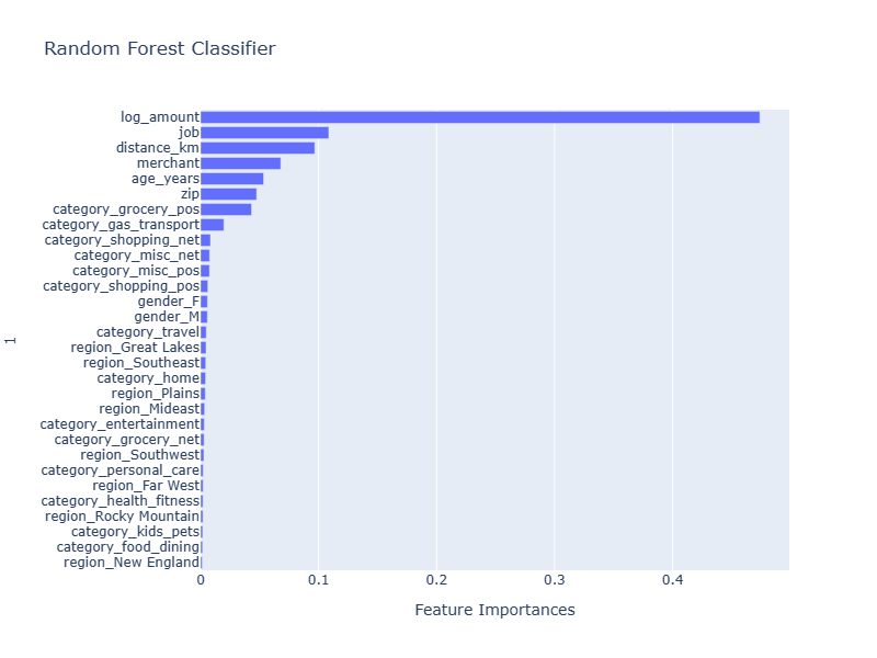
The random forest classifier generated the following feature importance which sheds light on the factors influencing the model prediction:
4. XGBoost with positive scaling of labels
| Confusion Matrix | Predicted Legitimate 0 | Predicted Fraudulent 1 | |
|---|---|---|---|
| Legitimate 0 | 137580 | 805 | |
| Fraudulent 1 | 50 | 495 | |
| Accuracy Score: 0.9938 | |||
| Balanced Accuracy Score: 0.9512 | |||
| Classification Report | |||
| Class | Precision | Recall | F1-score |
| 0 | 1.00 | 0.99 | 1.00 |
| 1 | 0.38 | 0.91 | 0.54 |
| Accuracy | 0.99 | ||
| Macro avg | 0.69 | 0.95 | 0.77 |
| Weighted avg | 1.00 | 0.99 | 1.00 |
The XGBoost model with its ability to accept a 'scale_pos_weight' parameter helps compensate for the class imbalance in the target variable. As a result, it performs much better at detecting fraudulent transactions than the other algorithms considered. The parameter 2'scale_pos_weights' is set to the ratio of negative transactions to positive transactions. (sum(negative_y)/sum(positive_y)) or 259.0 which when applied removes the imbalance in the target label during model fitting.
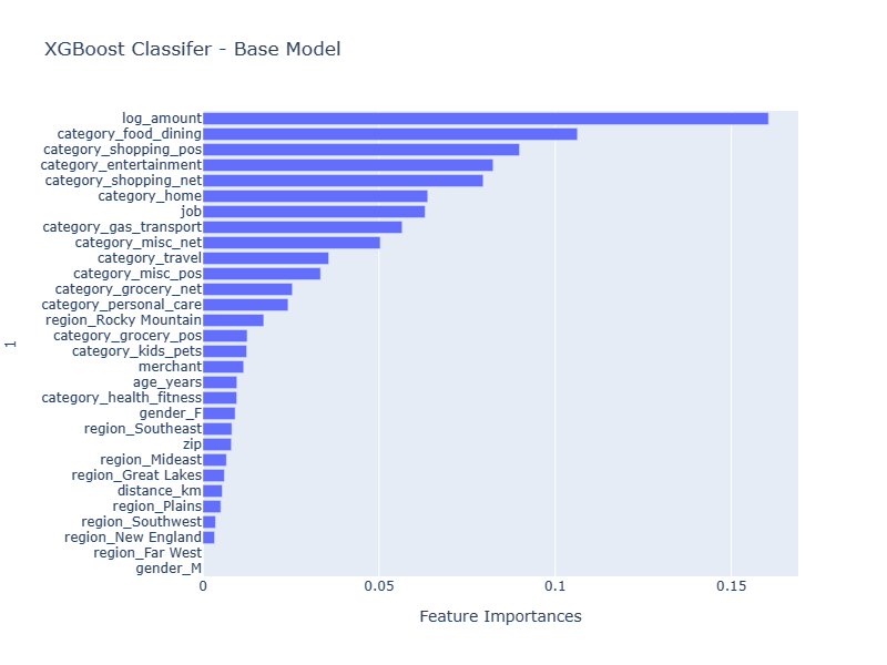
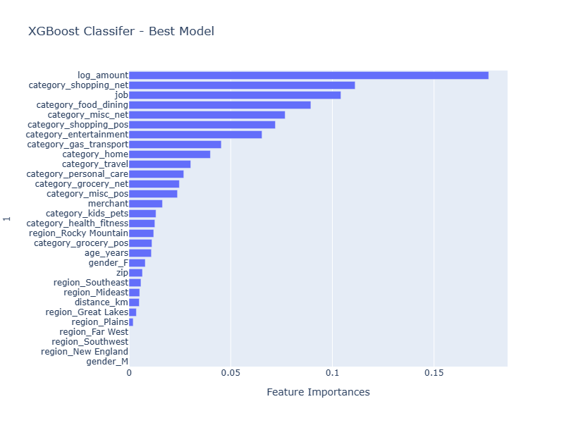
Note robustness of the XGBoost algorithm is evident when reviewing the relative importance of the features applied. XGBoost can reduce the impact of a feature to zero or nearly zero which can assist the scientist with feature engineering.
Part 5 Algorithm Selection
After reviewing the model results XGBoost was selected for hyper-parameter tuning because:
- XGBoost has facilities to address the imbalance in the target class.
- XGBoost has available a robust set of parameters for hyper-parameter-tuning.
- XGBoost showed the most performance in the objective metric (balanced accuracy) from the algorithms reviewed.
Part 6 Tuning XGBoost and selecting the best model.
The parameters selected to be tuned were:
- The number of boosting rounds to run (32,64,128,256,512)
- The maximum depth of the trees created (2, 4, 6, 8, 10, 12)
- This results in 30 distinct models being evaluated.
The results were as follows:
- From the 30 models run by the tuner, 6 (20%) of the models met the primary requirement of meeting 0.965 balanced accuracy.
- From the 6 models 3 (50%) met the requirement of being within 1 standard deviation of the model with the highest precision.
- Of these 3 models, the one that rendered the fastest prediction was selected as the BEST model.
The tuning objective was set to maximize the balance accuracy score and secondarily improve model precision. Precision was chosen in an attempt to minimize the rate of false positives.
| Confusion Matrix | Predicted Legitimate 0 | Predicted Fraudulent 1 | |
|---|---|---|---|
| Legitimate 0 | 135526 | 2859 | |
| Fraudulent 1 | 10 | 535 | |
| Accuracy Score: 0.9793 | |||
| Balanced Accuracy Score: 0.9805 | |||
| Classification Report | |||
| Class | Precision | Recall | F1-score |
| 0 | 1.00 | 0.98 | 0.99 |
| 1 | 0.16 | 0.98 | 0.27 |
| Accuracy | 0.98 | ||
| Macro avg | 0.58 | 0.98 | 0.63 |
| Weighted avg | 1.00 | 0.98 | 0.99 |
The tuned model exhibited significant improvement in balanced accuracy (0.03) when evaluated against the test dataset, surpassing the base XGBoost model. Notably, it demonstrated heightened sensitivity to fraudulent transactions compared to all other reviewed models. However, this performance gain came at the cost of precision: 84% of the predicted fraudulent transactions were false positives, representing a 22% increase from the base model. Importantly, this translated to only 2% of legitimate transactions being incorrectly flagged as fraudulent.
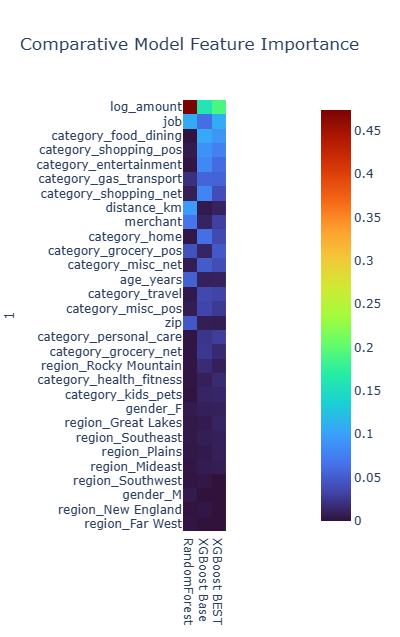
Comparative Feature Importance by Model
In our review of ensemble models, one consistent finding is that the log_amount of the transaction stands out as the most significant feature across all models. However, beyond this consistency, the importance of other features varies significantly from model to model. Notably, both the XGBoost Base Model and the XGBoost BEST model share several features that rank high in importance. To explore further, we could consider excluding some of the less significant features from the XGBoost BEST Model and assess whether this refinement leads to improved performance.
Final Conclusions
XGBoost, with its capability to adjust the weight of the positive target coupled with using balanced accuracy as the objective performance metric, serves as an effective framework for building binary classification models. This framework is particularly well-suited for classifying datasets with highly imbalanced target classes.
Footnotes:
[1]
Scikit Learn - Balanced Accuracy Score
[2]
XGBoost - Control of positive and negative weights
The following data science and visualization technologies were used in creating this analysis:


